Horror inspiring zooplankton, Ron Brown edition

Here are some zooplankton you wouldn’t want to meet in a dark alley! First up is Phronima sp. – a hyperiid amphipod that is said to the be the inspiration for the creature from the Alien movies. Females burrow into the bodies of unfortunate gelatinous zooplankton (like salps and jellyfish) to make a cozy home, then lay their eggs inside of the corpse. These creatures sound like they are straight out of a horror movie, but luckily for us they are only about the size of a quarter.

Photo 1: Phronima sp. captured in the 505 µm Bongo net. Photo credit: Caitlin Smoot.

Next up is a predatory copepod called Paraeuchaeta. The animals pictured below are around the size of a grain of rice. They prey on other copepods, but can prey on fish eggs too. We were lucky enough to collect female and male specimens in our 150 µm Bongo net. The male (bottom) uses his specialized fifth pair of swimming legs to transfer a sperm packet, or spermatophore, to the female’s genital segment in order to fertilize her eggs. The female from our net (top) has a spermatophore attached to her genital segment.

Photo 2: Female and male copepods (Paraeuchaeta sp.) collected in the 150 µm Bongo net. Photo credit: Caitlin Smoot.

Check out this link to the Plankton Chronicles for a great video of Phronima in action: http://www.planktonchronicles.org/en/episode/phronima-monsters-in-barrels

Until next time…be glad you’re not a salp!

-Caitlin

Albatross Flock!

We spotted a flock of Black-footed Albatross (Phoebastria nigripes) at the outermost station of the Yakutat line this morning. They are currently listed as endangered under the IUNC. Albatrosses are commonly seen in the Gulf of Alaska and along the Aleutian Islands during the summer months. Albatrosses are thought to be the reincarnated souls of sailors lost at sea in some cultures who watch over ships, so we had our own flock of guardian angels watching over us.  Photo by Jennifer Questel

Meet the CTD!

Our cruise has 3 major sources of data collection: the Burkolator, the Bongo nets, and the CTD. You can find more information on the Burkolator in this post, and we’ll cover the Bongo nets later in the week. This post will be dedicated to the CTD, the workhorse of the ship. CTD stands for Conductivity, Temperature, and Depth, which are the three sensors that you’ll find on every CTD. In addition to those sensors, each CTD rosette (the metal frame which holds the CTD) gets customized with a variety of other sensors based on the purpose of the cruise. On our CTD rosette we have (in addition to the conductivity and temperature sensors), a dissolved oxygen sensor, a fluorometer, a backscatter sensor, an altimeter, a UVP, and a LISST. Also on the rosette are Niskin bottles to collect discrete water samples. We’re taking several different types of water samples, including carbon, chlorophyll, and nutrients from the Niskin bottles. All of the Niskin bottles are controlled by a single carousel, which gets connected to a central computer called the “Fish” along with all of the sensors. The “Fish” is connected to the deck unit by a sea cable that runs inside of the winch cable, so we can get the data in real time. At the bottom of this post are photos of all of the instruments describing what they do and how they work, and there are some short videos of how we deploy & retrieve it!

The short version is that the CTD gives us a physical profile of the water column and discrete water samples from the depths we program into it. We do a CTD cast at every station we visit, with the ultimate goal of getting a “snap shot” of the Gulf of Alaska at this time of year. We’ll be able to match the CTD profiles to the biological data collected by the Bongos (more on that later!). The CTD & Bongo nets are the lifeblood of the cruise—they cannot be deployed by drones or autonomous gliders, and they are the only way to collect the discrete chemical & biological samples we need to run the breadth of measurements that we need to understand the physical and biological systems of this area. 

-Katie

Video 1- CTD Deployment (day). Morgan Ostendorf (PMEL/UW), Mark Bradley (NOAA OMAO) and Max Schoenfeld (UAF) deploy the CTD on the day shift. Taken by Kathryn Beaumont.

Video 2 –CTD Deployment (night). Julian Herndon (PMEL/UW) and Bill Potts (NOAA OMAO) deploy the CTD on the night shift. Taken by Kathryn Beaumont

Video 3 – CTD Retrieval. Morgan O. (PMEL/UW), Mark B. (NOAA OMAO) and Kathryn Beaumont (NMFS / UW) retrieve the CTD on the day shift. Taken by Kathryn Beaumont

                                          


Photo 1 – The CTD rosette being prepped for deployment by Mark B. (NOAA OMAO), Dan Naber (UAF) and Max S. (UAF). You can see that the Niskin bottles are cocked in this photo (the caps on the tops & bottoms of the bottles are pulled back. The bottles will be fired at certain depths (the caps will snap on) to collect discrete water samples. Photo by Kathryn Beaumont

The Niskin bottle carousel (top of the CTD) being prepped by Max S. (UAF). The caps are cocked by means of a nylon cord, which attaches to a firing pin on the carousel & keeps the caps open. The carousel is connected to the “Fish” computer, so the CTD operator can fire specific pins when the CTD reaches the correct depths. Generally the bottle samples are collected on the “upcast”, when the CTD is on its way back up to the surface. The “downcast” is reserved for getting a continuous physical profile of the water column, and then we stop at appropriate depths to collect water samples on the way up. Photo by Kathryn Beaumont 

Photo 3 – Whole CTD without cocked Niskin bottles. This is what the CTD looks like while we are in transit between stations. Photo by Kathryn Beaumont

Photo 4 – Carousel without cocked Niskin bottles. This is what the carousel looks like before the nylon cables get attached. Photo by Kathryn Beaumont

Photo 5 – Pump intakes, conductivity & DO probes. Our CTD has two different sets of pumps & conductivity, temperature and DO probes, a primary set and a secondary set (left and right respectively). The pump intakes are currently connected to syringes of DI water to keep the sensors from drying out and getting damaged. You can also see that the pumps and sensors are all connected to the top and bottom of the "Fish", the main brain of the CTD. Photo by Kathryn Beaumont

Photo 6 – Secondary pump, fluorimeter, and altimeter. The fluorimeter (black sensor) measures the amount of chlorophyll in the water as the CTD descends by reading certain wavelengths of light. The altimeter (silver sensor) pings the sea floor and tells us how close to the bottom the CTD is, which is very important so that we don’t crash the CTD into the sea floor! Photo by Kathryn Beaumont

Photo 7- Backscatter & primary pump. The backscatter (black sensor) reads the amount of reflected light as the CTD descends to get a measurement of turbidity.

Photo 8- The "Fish". This is the central computer which aggregates all of the sensor data and sends it back to the CTD operator via the sea cable, and also distributes the operator’s commands to the carousel and other instruments. Photo by Kathryn Beaumont

Photo 9 – Sea cable. The sea cable goes inside the winch cable to allow the CTD operator to control the instruments on the rosette as the CTD descends. Photo by Kathryn Beaumont

Photo 10 – UVP, which stands for Underwater Vision Profiler. This instrument takes greyscale photos of particles & organisms between 500 um and a few cm in diameter and also generates particle distribution for particles between 100um to ~3cm in diameter. Photo by Kathryn Beaumont

Photo 11 – LISST, which stands for Laser In Situ Scattering Transmission. This instrument uses laser backscattering to measure particle size distribution for sizes 2.5 um to 500 um.  Photo by Kathryn Beaumont

Photo 12 – Top down view of CTD. Photo by Kathryn Beaumont

Just finished the Dixon Entrance Transect!

Photo 1: Screenshot of transect map. The red circle with the cross is our current position, and the red and yellow circle is our destination. The triangles in the box mark the stations we just completed on the Dixon Entrance Transect!

We just finished our first transect, the Dixon Entrance Transect! This was our chance to learn how to work together, figure out where everything was on the ship, & get into a routine. Fortunately it all went pretty smoothly. We hit the first station around 1730 PDT yesterday (2015/07/16), and finished the last one around 1400 PDT today (2015/07/17). There were 8 in total; we started off shore and headed inland. Fortunately the first few stations were relatively far apart, so we had time to work out our sampling routine and get into a groove before we started getting slammed. Now that we are done with the Dixon Entrance transect, we are headed to the Prince of Wales Transect about 5 hours northwest of us (see the map above for our predicted path). Below are some photos of what happens at a station, from the CTD cast to the sample collection. Enjoy!

--Katie

Photo 2: We saw whales on the way to the transect! Photo credit Jennifer Questel

Photo 3: Our first CTD deployment! The CTD rosette is being stabilized by Mark Bradley (NOAA OMAO) and Morgan Ostendorf (PMEL/UW) as it descends, with Michael Lastinger (NOAA OMAO) assisting. Photo credit Jennifer Questel

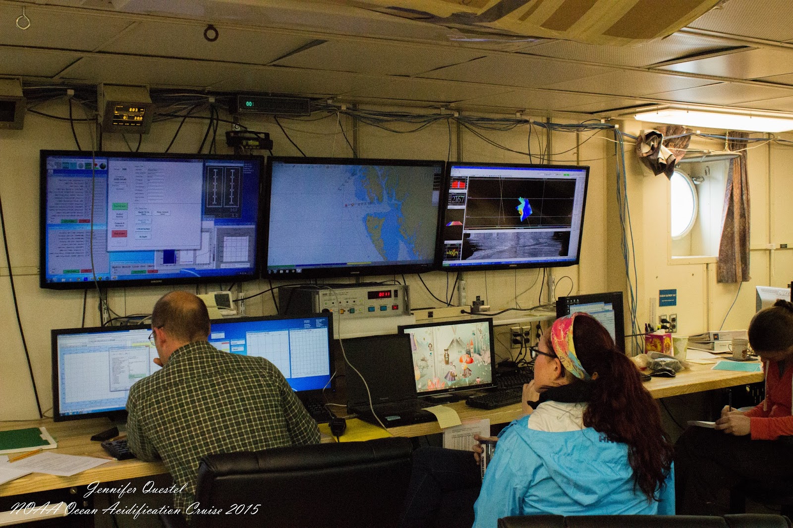
Photo 4: Inside the computer lab for the first CTD deployment. Wiley Evans (UAF/PMEL), Jessica Pretty (UAF), and Caitlin Smoot (UAF) are manning the screens. Photo credit Jennifer Questel

Photo 5: The CTD coming out of the water! That hook will be used to attach one of two lines to the CTD to stabilize it as we bring it back on deck. Photo credit Kathryn Beaumont

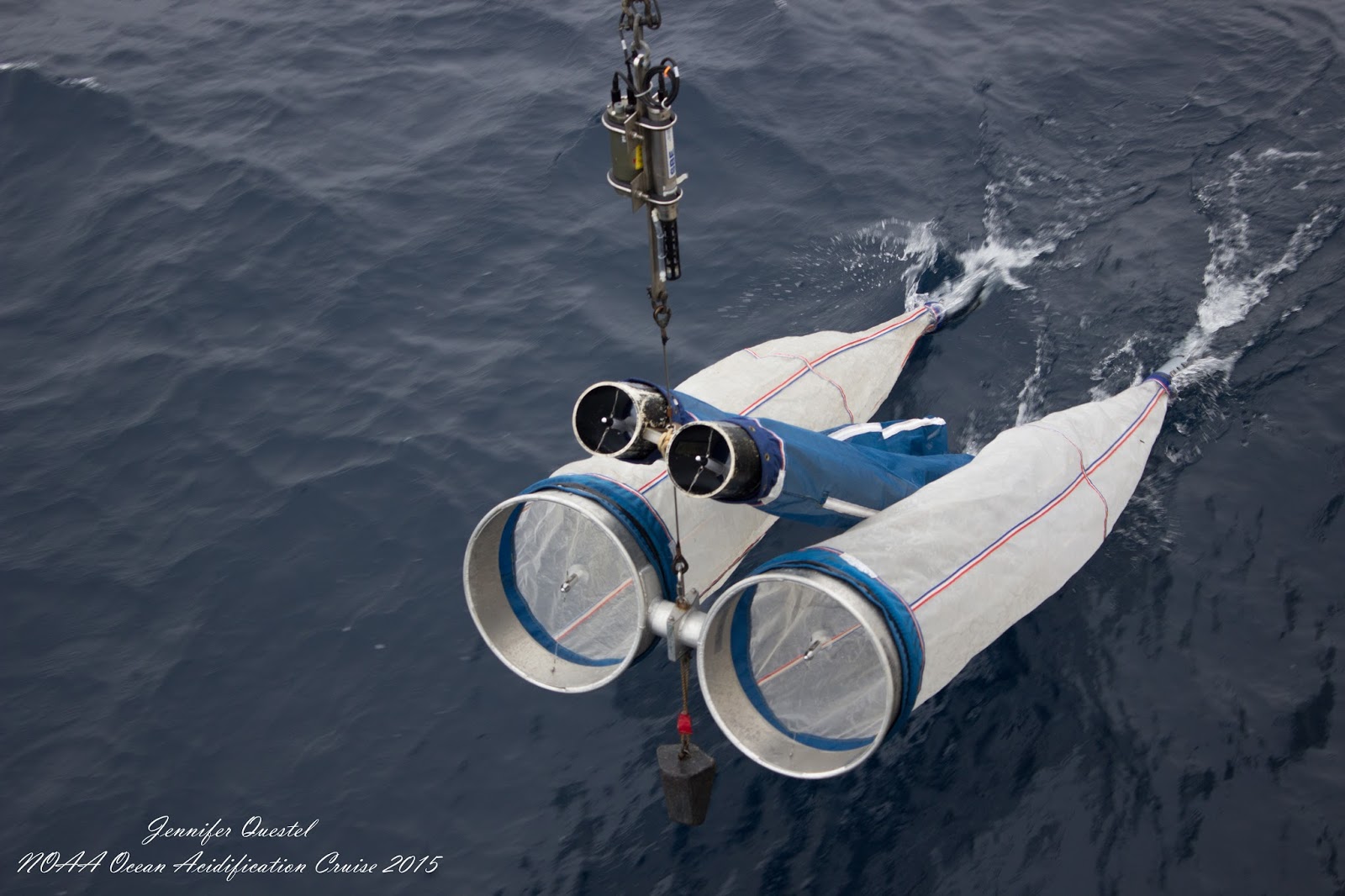
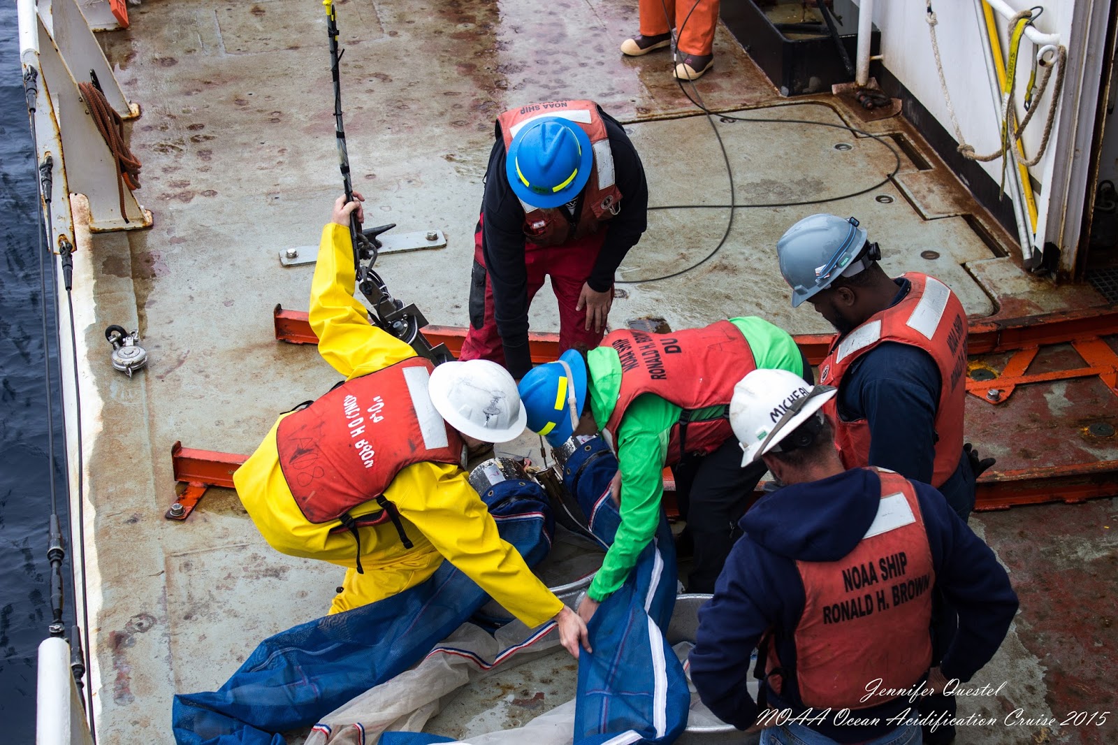
Photo 6: Prepping the Bongo nets for deployment. Mark B. (NOAA OMAO), Max Schoenfeld (UAF), Michael L. (Ron Brown), Jennifer Questel (UAF), and Kadarius Jones (NOAA OMAO). Photo credit Jennifer Questel

Photo 7: The bongo nets are being lowered into the water. The two little nets on top are 150nm mesh, and the two nets on the bottom are 505nm mesh. The instrument on the line above the nets tells us how deep the nets are as they get reeled out, and there are flow meters suspended in the center. Photo credit Jennifer Questel

Photo 8: Morgan O. (PMEL) taking a DIC sample from a Niskin bottle. Photo credit Jennifer Questel

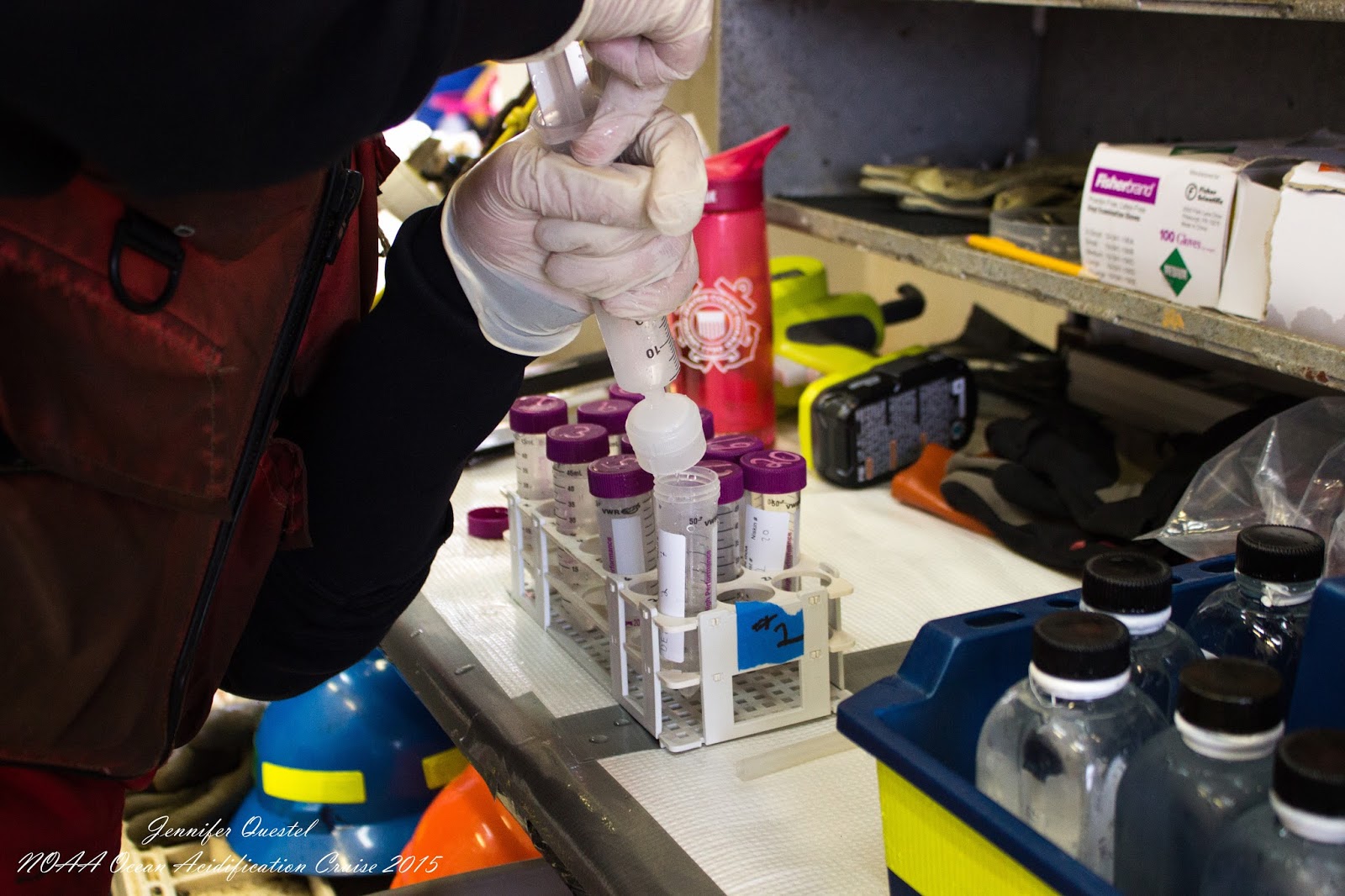
Photo 9: Max S. (UAF) taking filtered nutrient samples. The water is drawn into the syringe directly from the Niskin bottle, and then is pushed through a filter attachment into the sample vial. Photo credit Jennifer Questel 

Photo 10: Caitlin S. (UAF) and Kathryn Beaumont (NOAA NMFS/UW) running the sample from the 505nm bongo net cod end through a coarse sieve. Photo credit Jennifer Questel

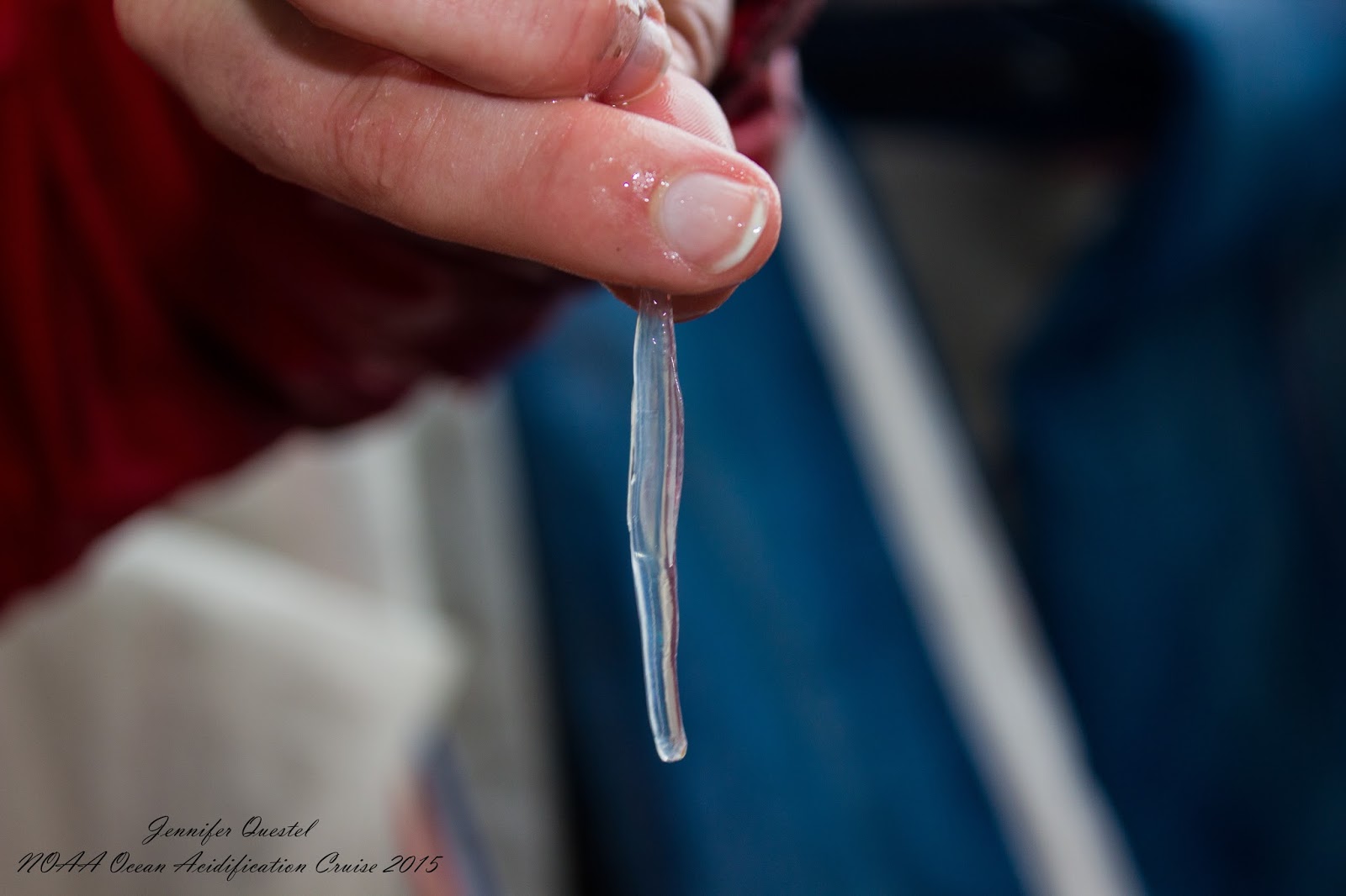
Photo 11: Caitlin S. (UAF) holding a chaetognath (arrow worm) from the sieve. Photo credit Jennifer Questel

Photo 12: Night shift in the computer lab. Jenn Q. (UAF) is catching a quick nap between stations. The night shift is 12am - 12pm, and the day shift is 12pm - 12am. Photo credit Jessica Pretty

Burkolator on the Brown: Our First OA Measurements

The first OA measurements we made once in U.S. waters (sadly there was no sampling in Canadian waters on the transit up to Alaska from Seattle due to a lack of clearance) are from a CO2 system known as a “Burkolator” (after designer Dr. Burke Hales, Oregon State University; Photo 1). This system will continuously sample surface seawater flowing through the ship during this cruise in the coastal Gulf of Alaska and the following cruise in the Bering Sea. The data from this system will provide a highly resolved snapshot of surface CO2 conditions along nearly half of the state of Alaska’s extensive coastline. We’re specifically interested in the saturation index of calcium carbonate; the mineral used by shelled marine organisms. The Burkolator is integrated with a series of ancillary sensors, such that the core CO2 system measurements we’re making are CO2 partial pressure (pCO2), total CO2 (TCO2), and pH (SeaFET). The system also tracks dissolved oxygen concentrations (SBE63), chlorophyll fluorescence (WETStar) and beam transmission related to the particle loads (C-Star). The combination of these measurements allows us to assess the physical and biological processes that shape the CO2 conditions in the surface water. An example of the data being collected and displayed in real-time is shown in Photo 2.

- Wiley Evans



Photo 1: The Burkolator installed on the NOAA Ship Ronald H. Brown. The various components are labeled and include: the control computer, electronics box, wet chemistry bench, liquid and gas standards, a bubble-typed equilibrator, SeaFET pH sensor, SBE63 dissolved oxygen sensor, C-Star beam transmissometer, and a WETStar chlorophyll fluorometer. Also shown is the Atlantic Oceanographic and Meteorological Laboratory (AOML) CO2 system that is permanently installed on the R. H. Brown and will provide a comparison dataset for the Burkolator. Photo taken by Wiley Evans





Photo 2: Example of the real-time data displayed by the Burkolator. This is a 4.5-hour window from July 17 showing pCO2 (white), saturation index for calcium carbonate (aragonite, blue), surface seawater temperature (red), salinity (green), and pH (purple). Photo taken by Wiley Evans

Welcome to our cruise blog!

Hello everyone,

Welcome to our cruise blog! This mission is part of the NOAA Ocean Acidification Monitoring Program. The OAP brings together a multi-faceted national network to understand and predict pH changes of the oceans and Great Lakes. Ocean Acidification (OA) refers to gradual decreases in ocean pH and other chemical changes caused primarily by uptake of excess atmospheric carbon dioxide. Human activity, like the burning of fossil fuels and land use change, is causing OA to proceed at a much faster rate than normal.

During the last decade, OA has become a pressing concern for many fisheries and ecosystems in vulnerable areas that already have naturally higher concentrations of CO2, like coastal areas, upwelling zones, and colder high latitude areas. To a certain extent, all of these vulnerabilities are characteristics of the Gulf of Alaska. On top of that, this area is home to a large commercial salmon fishing industry. Salmon feed extensively on pteropods, a tiny shelled organism that is highly vulnerable to ocean acidification.

Another chemical change occurring with ocean acidification is a reduction in carbonate ions, which pteropods use to build shells. When concentrations of carbonate are low enough, it becomes very difficult for pteropods to build shells, and eventually, existing shells start to dissolve.

On this mission, a multidisciplinary team is making broad-scale observations of pH and carbonate chemistry directly alongside biological monitoring. It’s a unique opportunity to see whether or not patterns in the biology are related to the chemistry of the water. It’s also the first time we’ve been able to survey the whole Gulf of Alaska coast at once. This is a really unique opportunity to get a gulf-wide ‘snapshot’ of the region’s carbonate chemistry during this time of year.

Throughout the mission, we’ll be blogging about our everyday activities, as well as highlighting a couple of the specific projects we’re pursuing. We are particularly encouraging our new sailors and young student scientists to share their experiences with you.

To start off, we have had excellent weather during our transit up from Seattle—bright sunshine during the day. We even passed a pod of humpback whales yesterday! After our long journey north, we should reach our first station at about 1700 PST.

Fair winds and following seas;

--Jessica